In the previous post of this series, we discussed single qubit gates. In this next instalment, we are going to explore gates that act on multiple qubits at once, thus completing the exploration of quantum circuit building. We are also going to slowly, but diligently uncover the underlying theoretical scheme towards one of the most bizarre concepts in quantum mechanics - entanglement, which is something that will be dedicating the next part to.

Mathematics and philosophy of multi qubit registers 🔗

Once the quantum computational system grows from a single to multiple qubits, we arrive at a concept of a compound quantum system. Greg Jaeger, in his excellent study of entanglement, reminds us of a mathematical framework in which such systems are embedded:

The Hilbert space of a compound quantum system is the tensor product of the Hilbert spaces of the subsystems. The pure-state space for a system of $N$ two-level systems is the Hilbert space $\mathcal{H}^{(N)} = \mathbb{C}^2\otimes\mathbb{C}^2\otimes…\otimes\mathbb{C}^2$.

As such, from the quantum information theory point of view, when dealing with multiple qubits, the overall state of the system is described not by a sum, but by a tensor product of all the individual qubit constituents (or, to be more formal, subsystems), represented below by $\psi_n$.

$$\ket{\psi} = \ket{\psi_1}\otimes\ket{\psi_2} … \otimes\ket{\psi_n}$$

As it was determined in the earlier parts of this series, quantum gates are represented by $2^n * 2^n$ sized unitary matrices, where $n$ stands for the number of qubits the gate acts on. This definition naturally implies that while single qubit matrices are $2$x$2$ in size, two-qubit gates are going to be $4$x$4$ matrices, representing a 4-dimensional abstract complex vector spaces, or more specifically, after Jaeger, Hilbert spaces. For example, for single qubits, the computational basis consists of two basic unit vectors

The tensor product of two qubits viewed in standard basis is:

We could extrapolate this calculations onto larger qubit registers using the exact same mathematics. At the time of writing, the largest available quantum computer was constructed by Google and consists of 53 qubits. Describing a complete state of such a system requires $2^{53}$ dimensional Hilbert space, and $2^{53}$ is a really large number - $9,007,199,254,740,992$.

Arkady Plotnitsky summarizes this situation in The Principles of Quantum Theory, From Planck’s Quanta to the Higgs Boson:

His [Heisenberg’s] new theory offers the possibility of predicting, in general probabilistically, the outcomes of quantum experiments, at the cost of abandoning the physical description or representation, however idealized, of the ultimate objects and processes considered. This cost was unacceptable to some, event to most, beginning with Einstein (…). The nature of the mathematics used, that of the infinite-dimensional Hilbert spaces over complex numbers, already makes it difficult to establish realist representations of physical processes.

Leaving the philosophical debates about the nature of reality aside for now, let’s consider the following two qubit system, where the two qubits are in states $\ket{\psi_1}$ and $\ket{\psi_2}$ and the probability amplitudes are $\alpha_1$, $\beta_1$ and $\alpha_2$, $\beta_2$ respectively. As thoroughly analyzed in the earlier parts of this series, each qubit can written as a linear combination of two basis states.

$$\ket{\psi_1} = \alpha_1\ket{0} + \beta_1\ket{1}$$
$$\ket{\psi_2} = \alpha_2\ket{0} + \beta_2\ket{1}$$

The state of this two qubit system is then expressed by the tensor product of $\ket{\psi_1}$ and $\ket{\psi_2}$:

$$\ket{\psi_1}\otimes\ket{\psi_2} = \alpha_1\alpha_2\ket{0}\ket{0} + \alpha_1\beta_2\ket{0}\ket{1}\ + \beta_1\alpha_2\ket{1}\ket{0} + \beta_1\beta_2\ket{1}\ket{1}$$

Additionally, in the Dirac braket notation, it is customary to merge the neighbouring kets into a single ket, to make the entire equation more succinct and readable:

$$\ket{\psi_1}\otimes\ket{\psi_2} = \alpha_1\alpha_2\ket{00} + \alpha_1\beta_2\ket{01}\ + \beta_1\alpha_2\ket{10} + \beta_1\beta_2\ket{11}$$

The above equation is also important because we will return to it when we look at entanglement. When working with multi-qubit registers, we can always combine single-qubit unitary transformations to produce a multi-qubit transformation (gate). This is done by expressing those transformations as tensor products of single qubit transformations. Following this rule, $X \otimes Z$ is the same as $X \otimes I$ followed by $I \otimes Z$, where $I$ is the identity gate.

The opposite, however, is not always possible - not every multi-qubit transformation can be decomposed into a set of single qubit ones. The reason behind this is, again, the embodiment of the weirdness of quantum phenomena - some of the subsystems (qubits) may be entangled, and thus their states are not possible to be expressed individually anymore. However, as mentioned, for now we are going to attempt to steer away from the depths of entanglement though, as we are going to dedicate the entire next post to it.

The CNOT Gate 🔗

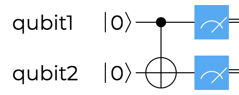
CNOT stands for a “controlled NOT”, which means it acts like the single qubit NOT ($X$) gate but in a conditional way, where the condition spans onto the second qubit. The gate is also often referred to as “controlled bitflip”. CNOT treats the first qubit as a so-called “control qubit” and the second one as a “target qubit”. Upon application of CNOT, the value of the control qubit doesn’t change, while target qubit may change conditionally - depending on the value of the control qubit. A partial counterpart to the logic behind CNOT in classical computing is the XOR operation, or the so called exclusive OR, because the change in the target qubit value upon measurement would correspond to the XOR logic.

For two classic bit inputs XOR logic returns $0$ when the two inputs are both $0$ or both $1$, and $1$ when the two input values differ - one is a $0$ and the other a $1$. Similarly, if we leave aside the quantum mechanical concept of a superposition and the complexities arising from that, and only imagine that the qubit can only be in one of the two basis states $\ket{0}$ and $\ket{1}$ (thus behaving like a classical bit), we can summarize the effect of CNOT gate accordingly - when the control qubit is $\ket{0}$, then the target qubit doesn’t change its value. However, when the control qubit is $\ket{1}$, the value of the target swapped is swapped - from $\ket{0}$ to $\ket{1}$ and vice versa.

$$\ket{00}\rightarrow\ket{00}$$
$$\ket{01}\rightarrow\ket{01}$$
$$\ket{10}\rightarrow\ket{11}$$
$$\ket{11}\rightarrow\ket{10}$$

CNOT is mathematically expressed using the following matrix:

At this point, it’s going to be beneficial to abandon purely theoretical deliberations and look at some Q# code. A word of qualification is in order though. In the three earlier posts of this series, we used a particular construct for our Q# programs - more specifically, a hybrid C# + Q# model, where C# provided a shell driver applications, and Q# contained quantum logic invoked from that application. Since then, the QDK, in one of the recent updates, shipped a new feature - standalone Q# command line applications. This feature allows us to use pure Q# programs, making the entire journey through quantum coding much more straight forward, as it eliminates the extra baggage of having to deal with an extra separate programming language. I blogged about this feature in detail on the Q# community blog recently, so I will skip the introduction to it here - I recommend however that you have a short look there.

A full example of a simmple Q# program that uses CNOT (from the $Microsoft.Quantum.Intrinsic$ namespace) against two qubits, and then measures the qubits to verify the results is shown below:

@EntryPoint()
operation Start() : Unit {
    
    Message("CNOT");
    ControlledNotSample(false, false); // |00>
    ControlledNotSample(false, true); // |01>
    ControlledNotSample(true, false); // |10>
    ControlledNotSample(true, true); // |11>   
}

operation ControlledNotSample(controlInitialState : Bool, targetInitialState : Bool) : Unit {
    using ((control, target) = (Qubit(), Qubit())) {
            PrepareQubitState(control, controlInitialState);
            PrepareQubitState(target, targetInitialState);

            CNOT(control, target);
            let resultControl = MResetZ(control);
            let resultTarget = MResetZ(target);
            Message("|" + (controlInitialState ? "1" | "0") + (targetInitialState ? "1" | "0") +">==>|" + (resultControl == One ? "1" | "0") + (resultTarget == One ? "1" | "0") +">");
    }
}

operation PrepareQubitState(qubit : Qubit, initialState : Bool) : Unit is Adj
{
    if (initialState) {
        X(qubit);
    }
}

In this sample, as mentioned, we only deal with qubits in the two orthogonal basis states $\ket{0}$ to $\ket{1}$. We always borrow (“allocate”, in the C# language) two qubits, and use them to apply the CNOT gate. The sample runs 4 times - for four different starting states $\ket{00}$, $\ket{01}$, $\ket{10}$ and $\ket{11}$. The $Message$ function prints the output to the console, and we keep track of the state transformations. What we should see is the following:

CNOT
|00>==>|00>
|01>==>|01>
|10>==>|11>
|11>==>|10>

This is of course as expected - the states $\ket{00}$ and $\ket{01}$ are left intact, while the states $\ket{10}$ and $\ket{11}$ result in the change in the target qubit value, along the lines of the classical XOR logic.

At this point it also worth mentioning that the notion of a “control qubit” and a “target qubit” is only an approximation of the real behavior of CNOT in quantum computing, and while helpful for high-level understanding, it should not be taken too literally. As it was discussed in part 1 of this series, measurements in quantum computing are basis dependent. Situation is the same with the effects of the CNOT gate. So far we were only discussing its behavior in the standard computational basis ($\ket{0},\ket{1}$), however, we could use the gate in a different basis, say, Hadamard basis ($\ket{+} ,\ket{-}$). In Hadamard basis, the notions of control and target qubits would appear to be effectively flipped, as it is the second qubit that remains unchanged, and the first one changes - conditionally - its state. The state transformations (without going into the mathematical proof) look the following:

$$\ket{++}\rightarrow\ket{++}$$
$$\ket{+-}\rightarrow\ket{-}$$
$$\ket{-+}\rightarrow\ket{-+}$$
$$\ket{-}\rightarrow\ket{+-}$$

CNOT generalization 🔗

CNOT can be viewed as a composite gate applying the $I$ transformation to the first qubit, and then the $X$ (“NOT”) to the second one. Taking this a step further, we can generalize it further by saying that we can construct any generic $CU$ gate, where the control remains unchanged and the target has $U$ applied to it.

Such generalizations are common in the quantum computing literature - for example Bob Sutor in his recent book Dancing with Qubits provides exhaustive information about constructing $CY$, $CZ$ or even $CR^Z_\phi$ gates. Q# does not intrinsically implement those gates, however it does provide a general purpose mechanism of creating general controlled unitary transformations via the $Controlled$ functor. A simple example of achieving CNOT functionality via $Controlled$ functor and a single qubit $X$ gate in Q# is shown below:

@EntryPoint()
operation Start() : Unit {
    
    Message("CNOT via functor");
    ControlledNotSampleFunctor(false, false); // |00>
    ControlledNotSampleFunctor(false, true); // |01>
    ControlledNotSampleFunctor(true, false); // |10>
    ControlledNotSampleFunctor(true, true); // |11>  
}

operation ControlledNotSampleFunctor(controlInitialState : Bool, targetInitialState : Bool) : Unit {
    using ((control, target) = (Qubit(), Qubit())) {
        PrepareQubitState(control, controlInitialState);
        PrepareQubitState(target, targetInitialState);
        Controlled X([control], target);
        let resultControl = MResetZ(control);
        let resultTarget = MResetZ(target);
        Message("|" + (controlInitialState ? "1" | "0") + (targetInitialState ? "1" | "0") +">==>|" + (resultControl == One ? "1" | "0") + (resultTarget == One ? "1" | "0") +">");
    }
}

operation PrepareQubitState(qubit : Qubit, initialState : Bool) : Unit is Adj
{
    if (initialState) {
        X(qubit);
    }
}

The output of this code is identical to the earlier one when we used the built-in $CNOT$ gate.

CNOT via functor
|00>==>|00>
|01>==>|01>
|10>==>|11>
|11>==>|10>

SWAP gate 🔗

SWAP gate is represented by:

And it transforms the state in the following manner:

$$\ket{00}\rightarrow\ket{00}$$
$$\ket{01}\rightarrow\ket{10}$$
$$\ket{10}\rightarrow\ket{01}$$
$$\ket{11}\rightarrow\ket{11}$$

Just like the CNOT gate, SWAP function in Q# can be found in the $Microsoft.Quantum.Intrinsic$ namespace, and not surprisingly, takes two qubits as arguments. An example of using the SWAP gate in Q# is shown in the snippet below.

@EntryPoint()
operation Start() : Unit {
    
    Message("SWAP");
    SwapSample(false, false); // |00>
    SwapSample(false, true); // |01>
    SwapSample(true, false); // |10>
    SwapSample(true, true); // |11>  
}

operation SwapSample(firstState : Bool, secondState : Bool) : Unit {
    using ((first, second) = (Qubit(), Qubit())) {
        PrepareQubitState(first, firstState);
        PrepareQubitState(second, secondState);

        SWAP(first, second);
        let resultFirst = MResetZ(first);
        let resultSecond = MResetZ(second);
        Message("|" + (firstState ? "1" | "0") + (secondState ? "1" | "0") +">==>|" + (resultFirst == One ? "1" | "0") + (resultSecond == One ? "1" | "0") +">");
    }
}

operation PrepareQubitState(qubit : Qubit, initialState : Bool) : Unit is Adj
{
    if (initialState) {
        X(qubit);
    }
}

The code is actually identical to our earlier CNOT sample - with the only exception being that we (no pun intended) swapped CNOT with SWAP. The output is inline with our expectations:

SWAP
|00>==>|00>
|01>==>|10>
|10>==>|01>
|11>==>|11>

Toffoli gate 🔗

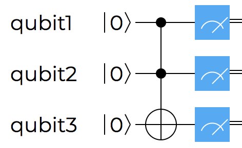
Toffoli gate is a three qubit gate that is an extrapolation of the CNOT gate logic onto three qubits. Logically, it follows similar XOR rules - with the first two qubits are both treated as control qubits, while the third plays the role of the target qubit. The first experimental realization of the gate in a trapped ion quantum computer was done in 2008 by a group at University of Innsbruck.

Since the first two qubits are controls, they never change and only if both of them are $1$, the final target state changes. In other words, the gate only swaps states $\ket{110}$ and $\ket{111}$ with each other and leaves all other states unchanged.

$$\ket{000}\rightarrow\ket{000}$$
$$\ket{001}\rightarrow\ket{001}$$
$$\ket{010}\rightarrow\ket{010}$$
$$\ket{011}\rightarrow\ket{011}$$
$$\ket{100}\rightarrow\ket{100}$$
$$\ket{101}\rightarrow\ket{101}$$
$$\ket{110}\rightarrow\ket{111}$$
$$\ket{111}\rightarrow\ket{110}$$

In Q# CCNOT is part of the $Microsoft.Quantum.Intrinsic$ namespace. It could also be constructed manually with the $Controlled$ functor.

@EntryPoint()
operation Start() : Unit {
    
    Message("SWAP with CNOTs");
    SwapSampleWithCnots(false, false); // |00>
    SwapSampleWithCnots(false, true); // |01>
    SwapSampleWithCnots(true, false); // |10>
    SwapSampleWithCnots(true, true); // |11>  
}

operation ToffoliSample(control1InitialState : Bool, control2InitialState : Bool, targetInitialState : Bool) : Unit {
    using ((control1, control2, target) = (Qubit(), Qubit(), Qubit())) {
        PrepareQubitState(control1, control1InitialState);
        PrepareQubitState(control2, control2InitialState);
        PrepareQubitState(target, targetInitialState);
        
        CCNOT(control1, control2, target);
        let resultControl1 = MResetZ(control1);
        let resultControl2 = MResetZ(control2);
        let resultTarget = MResetZ(target);
        Message("|" + (control1InitialState ? "1" | "0") + (control2InitialState ? "1" | "0") + (targetInitialState ? "1" | "0") +">==>|" + (resultControl1 == One ? "1" | "0") + (resultControl2 == One ? "1" | "0") + (resultTarget == One ? "1" | "0") +">");
    }
}

operation PrepareQubitState(qubit : Qubit, initialState : Bool) : Unit is Adj
{
    if (initialState) {
        X(qubit);
    }
}

The output, of course, aligns perfectly with what we expected.

Toffoli
|000>==>|000>
|001>==>|001>
|010>==>|010>
|100>==>|100>
|011>==>|011>
|101>==>|101>
|110>==>|111>
|111>==>|110>

Summary and entanglement 🔗

In this post we look at the mathematics behind multi-qubit gates, explored the CNOT, CCNOT and SWAP gates and identified a whole class of generic controlled gates. CNOT is definitely a very interesting gate from the algebraic perspective, and, as one of the universal quantum gates, is fundamentally important to the quantum information theory and quantum computing. However, since we explicitly qualified in the beginning of this post that we will ignore the superposition state of the control qubit, the CNOT behavior that we have seen so far is logical, deterministic and fully classical. Such context is useful to introduce the gate, but it also obfuscates the real reason why the gate is at the heart of quantum computing - and that’s the capability of the CNOT gate to entangle two qubits together. The next post in this series will be dedicated to entanglement, as we continue to dive deeper into the CNOT gate and the world of quantum computing.