In the world of quantum computing, generating true randomness is one of the most fundamental applications. But how do we know that a sequence of numbers is truly random and generated by a quantum process, rather than by a classical simulation or a pre-determined list?
In this post, we will explore a protocol to generate high-quality random numbers using a quantum computer, based on the recent paper Certified randomness amplification by dynamically probing remote random quantum states (Liu et al, arXiv:2511.03686, 2025). We will implement the core of this protocol using Q# for the quantum kernel and Python for the orchestration and verification, and then run it on a Q# simulator.
Protocol Overview 🔗
The protocol ensures that the randomness generated by a remote quantum device is genuine. It relies on the computational hardness of simulating random quantum circuits. The process involves several key steps:
- Challenge Generation
The client generates a random quantum circuit consisting of layers of random single-qubit gates and fixed two-qubit entangling gates. - Gate Streaming & Delayed Measurement
The client streams the single-qubit gates to the server. Crucially, the measurement basis for the final layer is revealed only at the very last moment, minimizing the time available for a malicious server to perform a classical simulation (spoofing). - Sampling
The quantum server executes the circuit and returns a bitstring sample within a strict time window. - Verification
The client verifies the randomness by computing the Linear Cross-Entropy Benchmarking (XEB)score. - Amplification
In the full protocol, the certified quantum randomness is combined with a weak random source to produce nearly perfect randomness.
The Quantum Kernel 🔗
The heart of our implementation is the Q# code that defines the quantum operations. The circuits used in this protocol have a specific structure:
- Initial State: $|0\rangle^{\otimes n}$
- Layers: Alternating layers of random single-qubit gates and fixed two-qubit gates (Rzz).
- Single-Qubit Gates: Drawn from the set ${ Z^p X^{1/2} Z^{-p} }$ where $p \in {-1, -3/4, \dots, 3/4}$. These are known as “phase-shifted X gates” and are chosen to avoid classical simulation shortcuts.
Here is the Q# implementation embedded in our Python script:
QSHARP_SOURCE = """
import Std.Math.*;
import Std.Arrays.*;
import Std.Diagnostics.*;
import Std.Measurement.*;

/// Applies the single-qubit gate used in the protocol: Z^p * X^(1/2) * Z^-p.
operation RandomSQGate(q : Qubit, p : Double) : Unit {
    // p corresponds to angles p * pi
    let angle = p * PI();

    // Z^-p
    Rz(-angle, q);

    // X^1/2 (pi/2 rotation)
    Rx(PI() / 2.0, q);

    // Z^p
    Rz(angle, q);
}

/// Applies the Random Circuit layers to the qubits.
/// Does NOT measure.
operation ApplyRandomCircuit(qubits : Qubit[], depth : Int, parameters : Double[], entanglingPairs : Int[]) : Unit {
    let nQubits = Length(qubits);
    let nPairsPerLayer = nQubits / 2;

    for d in 0..depth-1 {
        // 1. Layer of Random Single-Qubit Gates
        for q in 0..nQubits-1 {
            let paramIndex = d * nQubits + q;
            let p = parameters[paramIndex];
            RandomSQGate(qubits[q], p);
        }

        // 2. Layer of Entangling Gates (Rzz)
        for i in 0..nPairsPerLayer-1 {
            let baseIdx = (d * nPairsPerLayer + i) * 2;
            let q1 = entanglingPairs[baseIdx];
            let q2 = entanglingPairs[baseIdx + 1];

            Rzz(PI() / 2.0, qubits[q1], qubits[q2]);
        }
    }

    // 3. Final Layer (dynamic basis)
    let finalLayerStart = depth * nQubits;
    for q in 0..nQubits-1 {
        let p = parameters[finalLayerStart + q];
        RandomSQGate(qubits[q], p);
    }
}

/// Runs the random circuit sampling protocol and returns measurement results.
operation RunRandomCircuit(nQubits : Int, depth : Int, parameters : Double[], entanglingPairs : Int[]) : Result[] {
    use qubits = Qubit[nQubits];
    ApplyRandomCircuit(qubits, depth, parameters, entanglingPairs);

    // Measure and return results
    let results = MeasureEachZ(qubits);
    ResetAll(qubits);
    return results;
}
"""
Generating the Challenge 🔗
The client needs to generate the parameters for the random circuit. This includes the ‘p’ values for the single-qubit gates and the pairing for the entangling gates.
In this demonstration, we generate a new random pairing (topology) for every layer. The paper notes that for bandwidth optimization in the remote protocol, the two-qubit gate topology is typically fixed across circuits, but randomizing it here preserves the scrambling complexity required for certification.
def generate_circuit_data(num_qubits, depth, seed=None):
    """
    Generates the parameters and entangling pairs for the random circuit.

    Returns:
        - parameters: List of 'p' values for the single-qubit gates Z^p X^1/2 Z^-p.
        - entangling_pairs: List of qubit indices for the two-qubit gates.
    """
    rng = np.random.default_rng(seed)

    # Possible values for p as defined in the paper methods
    # p in {-1, -3/4, -1/2, ..., 3/4}
    p_values = np.linspace(-1, 0.75, 8)

    parameters = []
    entangling_pairs = []

    for d in range(depth):
        # 1. Layer of Random Single-Qubit Gates
        for q in range(num_qubits):
            p = rng.choice(p_values)
            parameters.append(float(p))

        # 2. Layer of Entangling Gates (Random Pairs)
        # Generate a random perfect matching
        qubits = np.arange(num_qubits)
        rng.shuffle(qubits)

        # Pair them up: (0,1), (2,3), etc.
        for i in range(0, num_qubits, 2):
            q1, q2 = int(qubits[i]), int(qubits[i+1])
            entangling_pairs.extend([q1, q2])

    # 3. Final Layer
    for q in range(num_qubits):
        p = rng.choice(p_values)
        parameters.append(float(p))

    return parameters, entangling_pairs
Ideal Simulation 🔗
To verify the output of the quantum computer, we need to compare the sampled bitstrings against the ideal probability distribution of the circuit. For small numbers of qubits, we can use a state vector simulator to compute the full probability distribution $|\psi|^2$.
def get_ideal_probabilities_qsharp(n_qubits, depth, parameters, entangling_pairs):
    """
    Uses Q# simulator to calculate the ideal state vector and probabilities.
    """
    # Reset simulator to ensure clean state (no accumulated qubits)
    qsharp.init()

    # Re-evaluate the Q# source code because init() cleared it
    qsharp.eval(QSHARP_SOURCE)

    qsharp.eval(f"use qs = Qubit[{n_qubits}];")
    qsharp.eval(f"ApplyRandomCircuit(qs, {depth}, {parameters}, {entangling_pairs});")

    dump = qsharp.dump_machine()
    qsharp.eval("ResetAll(qs);")

    # Extract probabilities from the dump
    amplitudes = dump.as_dense_state()
    probs = [abs(z)**2 for z in amplitudes]

    return probs
We also need a small utility to convert the Q# results into bitstrings:
def result_array_to_bitstring(result_array):
    """
    Converts Q# Result[] to a bitstring.
    Matches Q# DumpMachine endianness (Big Endian: q0 is MSB).
    """
    def map_res(r):
        s = str(r)
        if s == "One" or s == "1" or r == 1: return "1"
        return "0"

    return "".join(map_res(x) for x in result_array)
Certification (XEB) 🔗
The core of the protocol is the Linear Cross-Entropy Benchmarking (XEB) score. This score quantifies how well the experimental samples correlate with the ideal quantum distribution.
The XEB score is defined as: $$\text{XEB} = 2^n \langle P(x_i) \rangle - 1$$
where $n$ is the number of qubits, $x_i$ are the sampled bitstrings, and $P(x_i)$ is the ideal probability of observing bitstring $x_i$.
- XEB $\approx$ 1: Indicates the device is sampling from the ideal quantum distribution (high fidelity).
- XEB $\approx$ 0: Indicates the device is outputting uniform random noise or classical spoofing.
def calculate_xeb(sampled_bitstrings, ideal_probs):
    """
    Calculates Linear Cross-Entropy Benchmarking (XEB) score.
    """
    if not sampled_bitstrings:
        return 0.0

    n_qubits = len(sampled_bitstrings[0])
    N = 2**n_qubits

    observed_probs = []
    for b in sampled_bitstrings:
        idx = int(b, 2)
        if idx < len(ideal_probs):
            observed_probs.append(ideal_probs[idx])

    mean_prob = np.mean(observed_probs)
    xeb_score = (N * mean_prob) - 1
    return xeb_score

def calculate_theoretical_xeb(ideal_probs):
    """
    Calculates the theoretical expected XEB score for this specific circuit instance.
    Expected XEB = N * sum(p^2) - 1
    """
    N = len(ideal_probs)
    sum_sq = sum(p**2 for p in ideal_probs)
    return (N * sum_sq) - 1
Running the Protocol 🔗
Now, let’s put it all together. We will run the protocol with a small number of qubits ($N=4$) to demonstrate the process.
# --- Simulation Parameters ---
n_qubits = 4
depth = 8
shots = 10000

print(f"Running Certified Randomness Protocol with {n_qubits} qubits, depth {depth}...")

# 1. Generate Challenge (Parameters)
parameters, entangling_pairs = generate_circuit_data(n_qubits, depth, seed=42)
print("Challenge circuit generated.")

# 2. Simulate "Ideal" Quantum Computer (Q# Simulator)
print("Calculating ideal probabilities using Q# simulator...")
ideal_probs = get_ideal_probabilities_qsharp(n_qubits, depth, parameters, entangling_pairs)
print("Ideal probabilities calculated.")

# 3. Simulate "Real" Execution (Q# Sampling)
print(f"Executing on Q# simulator ({shots} shots)...")
from qsharp.code import RunRandomCircuit

sampled_bitstrings = []
for _ in range(shots):
    result = RunRandomCircuit(n_qubits, depth, parameters, entangling_pairs)
    bitstring = result_array_to_bitstring(result)
    sampled_bitstrings.append(bitstring)

print(f"Collected {len(sampled_bitstrings)} samples.")

# 4. Certification (XEB Calculation)
score = calculate_xeb(sampled_bitstrings, ideal_probs)
theoretical_score = calculate_theoretical_xeb(ideal_probs)

print("-" * 50)
print(f"XEB Score: {score:.4f}")
print(f"Theoretical Expected XEB (Infinite Shots): {theoretical_score:.4f}")
print("-" * 50)
When we run this, we get an XEB score that certifies the randomness. A score around 1.0 indicates ideal quantum behavior. If the score were close to 0, it would suggest classical noise or spoofing.
--------------------------------------------------
XEB Score: 1.2599
Theoretical Expected XEB (Infinite Shots): 1.2743
--------------------------------------------------
Interpretation:
1. XEB Score:
- ~1.0: Ideal Quantum Behavior (Perfect Fidelity) for large random circuits.
- ~0.0: Classical Randomness / Noise (Spoofing).
- > 0.1: Strong evidence of quantum interference.
- Your score (1.2599) indicates successful quantum certification.
- Note: For small systems (N=4) and specific circuit instances, scores > 1.0 are normal.
The score may exceed the theoretical expectation (1.2743) due to finite sampling noise (10000 shots).
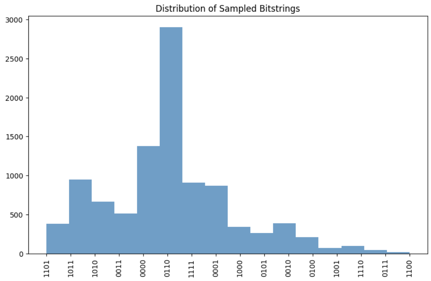
2. Histogram Shape:
- Quantum: 'Spiky' (Porter-Thomas distribution). Some outcomes are very frequent, others rare.
- Classical: Flat/Uniform. All outcomes appear with roughly equal frequency.
>>> SUCCESS: Randomness is certified quantum! <<<
And the histogram of sampled bitstrings could look like this (it would differ from run to run, but generally shows the “spiky” distribution):
Summary 🔗
In the full protocol described in the paper, the certified randomness obtained above is not the final output. It serves as a high-quality seed. The certified samples are combined with a weak random source using a “Two-Source Extractor” to produce a nearly perfect random seed, which is then amplified.
This two-step process allows for “Certified Randomness Amplification”, turning a weak, potentially biased source into a strong, certified random source using the quantum computer as a catalyst.
The source code for this post is available on GitHub. Merry Christmas and happy quantum computing! 🎄