If you visited this blog before, chances are you are familiar with Q# Bridge, a library that I have been working on for quite a while, that allows you to run Q# quantum simulations and access a number of Q# compiler/QDK features from multiple popular high-level languages such as C#, Swift, Python and Kotlin.
Today, I would like to shortly talk about a brand new feature in the library - the ability to generate Quantikz LaTeX circuits from Q# source code.
Motivation and background 🔗
When writing quantum computing papers, reports or other content, it is usually necessary to include circuit diagrams to illustrate quantum algorithms. When using LaTeX as your typesetting system, a de facto standard approach is to rely on the Quantikz package. It provides a simple yet powerful syntax for creating quantum circuit diagrams. However, manually creating these diagrams can be tedious and error-prone, especially for complex circuits.
Moreover, if you are already writing your quantum code in Q#, it would be great to be able to automatically generate the corresponding Quantikz diagrams directly from your Q# code.
This is exactly the problem that the new feature in Q# Bridge aims to solve. By leveraging the Q# compiler’s ability to analyze Q# code, and decompose it into a generic circuit representation, we can automatically generate Quantikz LaTeX code that accurately represents the quantum circuit described by the Q# operation.
Trying this out 🔗
The feature is available in the latest version of Q# Bridge - 0.2.1, and available from all supported languages. The usage is super simple. Here is a Jupyter Notebook example in Python.
Let’s start by installing the dependencies:
qsharp_bridge @ https://github.com/qsharp-community/qsharp-bridge/releases/download/0.2.1/qsharp_bridge-0.2.1-py3-none-linux_x86_64.whl; sys_platform == "linux"
qsharp_bridge @ https://github.com/qsharp-community/qsharp-bridge/releases/download/0.2.1/qsharp_bridge-0.2.1-py3-none-macosx_11_0_universal2.whl; sys_platform == "darwin"
qsharp_bridge @ https://github.com/qsharp-community/qsharp-bridge/releases/download/0.2.1/qsharp_bridge-0.2.1-py3-none-win_amd64.whl; sys_platform == "win32" and platform_machine == "AMD64"
qsharp_bridge @ https://github.com/qsharp-community/qsharp-bridge/releases/download/0.2.1/qsharp_bridge-0.2.1-py3-none-win_arm64.whl; sys_platform == "win32" and platform_machine == "ARM64"
jupyter-tikz
We only need Q# Bridge (distributed via a wheel from Github here) for circuit generation and the jupyter-tikz package for visualization - the core qsharp packages are not necessary for this feature to work.
First, we will import the library and all the other necessary packages and types. TeX rendering needs to work properly, so make sure that the TeX binaries are in the PATH (MacOS in my case):
from qsharp_bridge import *
from IPython.core.getipython import get_ipython
from IPython.core.interactiveshell import InteractiveShell

# Ensure that TeX binaries are in the PATH for LaTeX rendering
os.environ["PATH"] += os.pathsep + "/Library/TeX/texbin"
Next, let’s load the Jupyter TikZ extension.
%load_ext jupyter_tikz
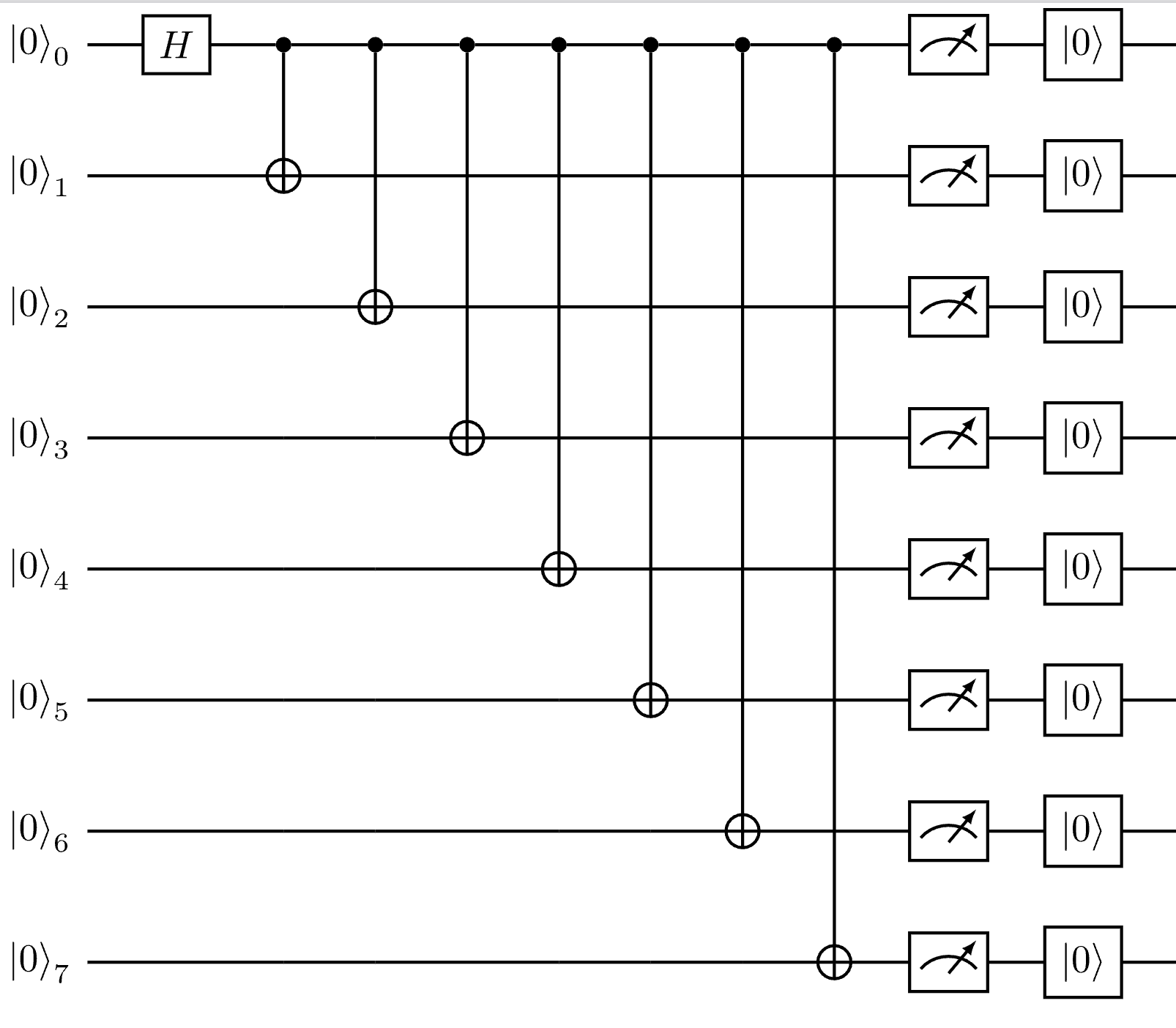
Now we can write some Q# code. This will be the Q# code for which we will generate a circuit diagram. We will set up two test code snippets - one that consists of a single operation, and another that has an operation calling another operation (this will become relevant in a moment).
code_1 = """
operation Main() : Result[] {
    use qubits = Qubit[8];

    // apply Hadamard gate to the first qubit
    H(qubits[0]);

    // apply CNOT gates to create entanglement
    for qubit in qubits[1..Length(qubits) - 1] {
        CNOT(qubits[0], qubit);
    }

    // return measurement results
    MResetEachZ(qubits)
}
"""

code_2 = """
namespace MyQuantumApp {
    @EntryPoint()
    operation Run() : (Result, Result) {
        use (control, target) = (Qubit(), Qubit());
        PrepareBellState(control, target);

        let resultControl = MResetZ(control);
        let resultTarget = MResetZ(target);
        return (resultControl, resultTarget);
    }

    operation PrepareBellState(q1 : Qubit, q2: Qubit) : Unit {
        H(q1);
        CNOT(q1, q2);
    }
}
"""
Once the Q# code is written, we can use the quantikz function from Q# Bridge to generate the Quantikiz LaTeX code:
quantikz_diagram_1 = quantikz(code_1, options=QuantikzGenerationOptions(group_by_scope=False))
quantikz_diagram_2 = quantikz(code_2, options=QuantikzGenerationOptions(group_by_scope=False))

# for debugging, display the generated LaTeX code
print(quantikz_diagram_1)
print(quantikz_diagram_2)
The output at this point will be the LaTeX code representing the quantum circuits. It should be something like this:
\begin{quantikz}
\lstick{$\ket{0}_{0}$} & \gate{H} & \ctrl{1} & \ctrl{2} & \ctrl{3} & \ctrl{4} & \ctrl{5} & \ctrl{6} & \ctrl{7} & \meter{} & \gate{\ket{0}} & \qw \\
\lstick{$\ket{0}_{1}$} & \qw & \targ{} & \qw & \qw & \qw & \qw & \qw & \qw & \meter{} & \gate{\ket{0}} & \qw \\
\lstick{$\ket{0}_{2}$} & \qw & \qw & \targ{} & \qw & \qw & \qw & \qw & \qw & \meter{} & \gate{\ket{0}} & \qw \\
\lstick{$\ket{0}_{3}$} & \qw & \qw & \qw & \targ{} & \qw & \qw & \qw & \qw & \meter{} & \gate{\ket{0}} & \qw \\
\lstick{$\ket{0}_{4}$} & \qw & \qw & \qw & \qw & \targ{} & \qw & \qw & \qw & \meter{} & \gate{\ket{0}} & \qw \\
\lstick{$\ket{0}_{5}$} & \qw & \qw & \qw & \qw & \qw & \targ{} & \qw & \qw & \meter{} & \gate{\ket{0}} & \qw \\
\lstick{$\ket{0}_{6}$} & \qw & \qw & \qw & \qw & \qw & \qw & \targ{} & \qw & \meter{} & \gate{\ket{0}} & \qw \\
\lstick{$\ket{0}_{7}$} & \qw & \qw & \qw & \qw & \qw & \qw & \qw & \targ{} & \meter{} & \gate{\ket{0}} & \qw \\
\end{quantikz}

\begin{quantikz}
\lstick{$\ket{0}_{0}$} & \gate{H} & \ctrl{1} & \meter{} & \gate{\ket{0}} & \qw \\
\lstick{$\ket{0}_{1}$} & \qw & \targ{} & \meter{} & \gate{\ket{0}} & \qw \\
\end{quantikz}
We can now use the TikZ extension to render a PDF from the LaTeX code generated by Q# Bridge to verify the output.
shell = get_ipython()
assert shell is not None

shell.run_cell_magic('tikz', '-l quantikz', quantikz_diagram_1)
And the other one:
shell = get_ipython()
assert shell is not None

shell.run_cell_magic('tikz', '-l quantikz', quantikz_diagram_2)
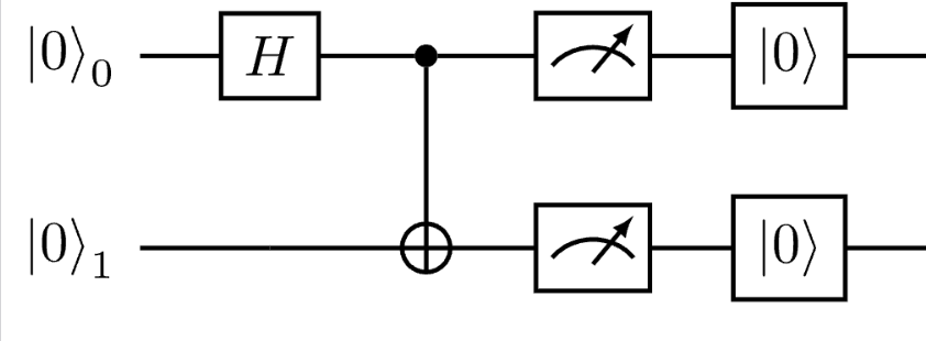
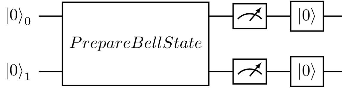
Notice how the two-operation sample was actually decomposed into its constituent individual gates in the generated diagram - this is because we set group_by_scope to False in the QuantikzGenerationOptions when generating the diagrams. Q# compiler (and, by extension, Q# Bridge) can also group gates on the circuit into groups scoped by an operation. In our case that would mean a large single block representing PrepareBellState.
So let’s set group_by_scope of the QuantikzGenerationOptions to True and pass that into the quantikz function - and see how the generated diagram changes.
quantikz_diagram_3 = quantikz(code_2, options=QuantikzGenerationOptions(group_by_scope=True))

# for debugging, display the generated LaTeX code
print(quantikz_diagram_3)

shell = get_ipython()
assert shell is not None

shell.run_cell_magic('tikz', '-l quantikz', quantikz_diagram_3)
This would now produce the quantikz circuit where the PrepareBellState operation is represented as a single block in the circuit diagram and no longer decomposed into individual gates.
\begin{quantikz}
\lstick{$\ket{0}_{0}$} & \gate[wires=2]{PrepareBellState} & \meter{} & \gate{\ket{0}} & \qw \\
\lstick{$\ket{0}_{1}$} & \qw & \meter{} & \gate{\ket{0}} & \qw \\
\end{quantikz}
When rendered, this would look like this:
Conclusion 🔗
Well that’s it! As you can see, generating Quantikz LaTeX circuits from Q# code using Q# Bridge is super easy and can save you a lot of time when preparing documents that require quantum circuit diagrams. You can find the demo notebook with the above code samples and more examples in the Q# Bridge repository.
Have fun!