In the last post in this series we dove deep into the mathematics and usage examples of multi-qubit gates, with special attention paid to one of the most critical gates in quantum computing, the CNOT gate.

In today’s post we are going to explore the wonders of entanglement - a core concept of quantum mechanics and a critical idea for quantum computing, where it is obtained via the application of the CNOT gate.

EPR pairs 🔗

The term “entanglement” was first introduced by Erwin Schrödinger in his “cat-paradox” paper “Die gegenwärtige Situation in der Quantenmechanik” (English translation is available here).

According to Schrödinger, with entangled states, we can no longer use the tensor products of the subsystem state vectors to describe the overall system state. In fact, for all intents and purposes, we can say that the individual states do not exist anymore as independent entities. Blanchard and Fröhlich describe this particularly troubling observation in their in-depth study of weird and counter-intuitive concepts of quantum mechanics:

If a quantum system consists of various parts, it is the total state that is primary. Two entangled electrons may have a definite total spin value in each direction, but no one of the two electrons has a definite spin value in itself in any direction. The components stand in a certain relation, but the total state of the composite system cannot be derived from the non-relational properties of these components. In contrast to classical objects, quantum objects are not characterized by intrinsic properties but by being part of more comprehensive systems.

In 1935, three physicists - Albert Einstein, Boris Podolsky, and Nathan Rosen, in a paper Can Quantum-Mechanical Description of Physical Reality be Considered Complete?, extended the work of Schrödinger, and described a paradox related to an entangled pair of particles. They realized that by exploring the correlations of the entangled pair, one can simultaneously predict exact definite values of properties quantum object even when it is disallowed by the uncertainty principle. This, according to the authors, proved that quantum mechanics is either incomplete or incorrect. Due to their work, entangled pairs of particles became commonly known as EPR pairs.

Arkady Plotnitsky in Epistemology and Probability, explains that the EPR paper reasoning, is in fact, subtly incorrect.

“in the problem in question we are not dealing with a single specified experimental arrangement, but are referring to two different, mutually exclusive arrangements”. (…) In the EPR case, we can predict with probability equal to unity the first quantity in question—say, the value of the position variable—for the second object, $S_{12}$, of a given EPR pair ($S_{11}$, $S_{12}$).We can then predict the second quantity—the value of the momentum variable—for the second object, $S_{22}$, of, unavoidably, another, “identically prepared” EPR pair ($S_{21}$, $S_{22}$). However, we cannot coordinate these predictions in such a way that they could be considered as pertaining to two identically prepared objects in the way this could be done in classical physics. This is not possible since the necessary intermediate measurements would, in general, give us different data.

Mathematics of entanglement 🔗

At purely theoretical level, we can speak of a system being in an entangled state, when it cannot be described by the individual states of its subsystems. As defined in the last post, given two separate qubit states $\ket{\psi_1}$ and $\ket{\psi_2}$:

$$\ket{\psi_1} = \alpha_1\ket{0} + \beta_1\ket{1}$$
$$\ket{\psi_2} = \alpha_2\ket{0} + \beta_2\ket{1}$$

The overall state of such composite system, when it is in an unentangled state, can be decomposed and expressed by the tensor product of the subsystems:

$$\ket{\psi} = \ket{\psi_1}\otimes\ket{\psi_2} = \alpha_1\alpha_2\ket{00} \ + \alpha_1\beta_2\ket{01} + \ \beta_1\alpha_2\ket{10} + \beta_1\beta_2\ket{11}$$

This is algebraically understandable and in itself doesn’t necessarily seem indicative of anything suspicious yet. It is, however, a good place to set off on the quest of searching for entanglement. Therefore, let’s consider the following quantum circuit, consisting of two gates are already familiar with, $CNOT$ and $H$, called the Bell circuit:

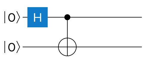
It is a two qubit circuit, and in the example above both input qubits start in $\ket{0}$ state (which we could write using the shorthand Dirac notation $\ket{00}$). The circuit uses a regular $CNOT$ gate, except the control qubit passes through the Hadamard gate first. As we already know, the $H$ gate will force the qubit state into a uniform linear superposition. We can now calculate the output of this gate:

Next thing to do would be to compare the output of the Bell circuit to the generalized description of a two-qubit system:

$$\alpha_1\alpha_2\ket{00} + \alpha_1\beta_2\ket{01} + \beta_1\alpha_2\ket{10} + \beta_1\beta_2\ket{11} = \ \frac{1}{\sqrt{2}}(\ket{00} + \ket{11})$$

This is starting to get a little more problematic. Notice that in the resulting state, the amplitude, and thus, per Born rule, the probability of receiving the states $\ket{01}$ or $\ket{10}$ are both $0$ for us. Given this information, we know that $\alpha_1\beta_2 = 0$ and $\beta_1\alpha_2 = 0$. This naturally implies that either $\alpha_1\alpha_2 = 0$ or $\beta_1\beta_2 = 0$ is also true, which is not the case - since both of these are explicitly non-zero. And this is the mathematical gist of entanglement - we cannot decompose an entangled qubit state into a tensor product of the individual qubit states. Moreover, upon measurement, we can only ever end up with $\ket{00}$ and $\ket{11}$, which implies that if we receive $\ket{0}$ when measuring the first qubit, the second is guaranteed to be $\ket{0}$ too, while if the first one produces $\ket{1}$ on measurement, we will certainly get $\ket{1}$ on the other one - provided the measurements are always done in the same basis, in this case in the computational basis, Pauli Z.

The state $\frac{1}{\sqrt{2}}(\ket{00} + \ket{11})$ is the so called Bell state, or to be more precise, one of the four Bell states, describing maximally entangled particles. In quantum mechanics their role, just like the role of entanglement in general, has historically been seen as more of a curiosity, relevant mainly for theorists. It is also worth noting that such pure simple biparticle states are rather an exception in nature - much complex systems emerge quickly. The role of entanglement, however, grew dramatically via the advent of quantum information theory, and the Bell states are fundamentally important in quantum computing, as they form the core concept around the possible quantum-over-classical computational advantage. This way they are often a key component for various quantum computing algorithms. The particular Bell state above is normally described by a symbol $\ket{\Phi^+}$ and we obtain it when the input states (also known as the input register) is $\ket{00}$.

All four of the Bell states are listed below, and they can be produced depending on the input to the Bell circuit. Together, they form an orthonormal basis for a two-qubit system:

$$\ket{00} \rightarrow \frac{1}{\sqrt{2}}(\ket{00} + \ket{11}) = \ket{\Phi^+}$$
$$\ket{10} \rightarrow \frac{1}{\sqrt{2}}(\ket{00} - \ket{11}) = \ket{\Phi^-}$$
$$\ket{01} \rightarrow \frac{1}{\sqrt{2}}(\ket{01} + \ket{10}) = \ket{\Psi^+}$$
$$\ket{11} \rightarrow \frac{1}{\sqrt{2}}(\ket{01} - \ket{10}) = \ket{\Psi^-}$$

It is also worth noting, that while the notion of superposition is basis-dependent - a qubit might be in superposition with respect to some bases, but not to other, something we covered in part 2 of this series - and that the basis choice would naturally impact measurement results of entanglement qubit, the notion of basis choice doesn’t impact entanglement itself. The measurement of both qubits using the same basis - any basis, no necessarily the Pauli Z - is however mandatory to observe the correlated results. This characteristic of entanglement is critical in the study and research of quantum cryptography.

Entanglement in Q# 🔗

We can of course use Q# to further explore and verify the properties of entangled quantum states. In principle such exercise would not be much different from the earlier work done in this series - as we only need the $H$ and $CNOT$ to produce a Bell state. This could be done by the following sequence of gate operations, where $control$ and $target$ represent two borrowed qubits.

H(control);
CNOT(control, target);

Q#, being a higher level language than a bare bones implementation of gate semantics, also offers a shortcut convenience operation to prepare a Bell state. This operation, $PrepareEntangledState$, is available in the $Microsoft.Quantum.Preparation$ namespace and allows us to entangle an arbitrary number of qubits. We could replace the above sequence of $H$ and $CNOT$ calls with a simple:

PrepareEntangledState([control], [target]);

Please pay attention to the array syntax - even though in our case we use just a single control and target qubits - to produce a classic singlet Bell state - it is possible to create more sophisticated entangled states too.

And example of a program initializing and measuring a Bell state is shown below. The operation is repeated a thousand times to help us develop a statistical understanding of what is going on. To do so, we will track how many times the resulting measurements on both the control and target qubit produce the four possible outcomes - $\ket{00}$, $\ket{01}$, $\ket{10}$ and $\ket{11}$. Additionally, we want to check how many times the measurement along the Z-axis of control qubit and target qubit agree with each other - to verify whether we really encounter the entanglement phenomenon and whether we can spot any statistical patterns in our results. The code below uses $PrepareQubitState$ operation that we defined in the last post, to flip $\ket{0}$ to $\ket{1}$, should out input register require so - this allows us to arbitrarily prepare qubits with $\ket{0}$ or $\ket{1}$ initial states. Since in a moment we shall try different Pauli bases for measurement, those are also exposed as input into the operation.

operation BellState(controlInitialState : Bool, targetInitialState : Bool, controlMeasurementBasis : Pauli, targetMeasureMeasurementBasis : Pauli) : Unit {
    mutable matchingMeasurement = 0;
    mutable zeroZero = 0;
    mutable zeroOne = 0;
    mutable oneZero = 0;
    mutable oneOne = 0;

    for (run in 0..999) {
        using ((control, target) = (Qubit(), Qubit())) {
                   // prepare |0> or |1> initial state
                PrepareQubitState(control, controlInitialState);
                PrepareQubitState(target, targetInitialState);

                PrepareEntangledState([control], [target]);
                
                let resultControl = Measure([controlMeasurementBasis], [control]);
                let resultTarget = Measure([targetMeasureMeasurementBasis], [target]);
                ResetAll([control, target]);

                set zeroZero += resultControl == Zero and resultTarget == Zero ? 1 | 0;
                set zeroOne += resultControl == Zero and resultTarget == One ? 1 | 0;
                set oneZero += resultControl == One and resultTarget == Zero ? 1 | 0;
                set oneOne += resultControl == One and resultTarget == One ? 1 | 0;
                set matchingMeasurement += resultControl == resultTarget ? 1 | 0;
        }
    }
    
    Message("Initial system state: |" + (controlInitialState ? "1" | "0") + (targetInitialState ? "1" | "0") +">");
    Message("|00>: " + IntAsString(zeroZero));
    Message("|01>: " + IntAsString(zeroOne));
    Message("|10>: " + IntAsString(oneZero));
    Message("|11>: " + IntAsString(oneOne));
    Message("Measurements of two qubits matched: " + IntAsString(matchingMeasurement));
}

We can now execute this code above and produce the Bell state $\Phi^+$. To do so, we shall initialize the input register to system state $\ket{00}$ and we will then follow with coordinated but independent measurements along the Z-axis ($PauliZ$ basis), using the following $EntryPoint$ operation:

namespace BellStateExample {

    open Microsoft.Quantum.Canon;
    open Microsoft.Quantum.Intrinsic;
    open Microsoft.Quantum.Measurement;
    open Microsoft.Quantum.Convert;
    open Microsoft.Quantum.Preparation;
    
    @EntryPoint()
    operation Start() : Unit {
        Message("Measuring control qubit in PauliZ and target qubit in PauliZ");
        BellState(false, false, PauliZ, PauliZ); // |00>
    }
}

The result should be the following, or approximately similar, since we are dealing with statistically varying results, output in the terminal:

Measuring control qubit in PauliZ and target qubit in PauliZ
Initial system state: |00>
|00>: 503
|01>: 0
|10>: 0
|11>: 497
Measurements of two qubits matched: 1000

The result confirms that just as predicted by quantum mechanics in the $\ket{\Phi^+} = \frac{1}{\sqrt{2}}(\ket{00} + \ket{11})$ Bell state, the two qubits became maximally entangled. The measurements never result in $\ket{01}$ or $\ket{10}$, but, with equal probability only $\ket{00}$ or $\ket{11}$. It follows that the measurements of the two qubits always agree with each other. Let’s now run the code for the other opposite Bell state $\Phi^-$. As we already algebraically determined, we can obtain the state $\ket{\Phi^-} = \frac{1}{\sqrt{2}}(\ket{00} - \ket{11})$ when starting with the input register of $\ket{10}$. Since the only difference between $\ket{\Phi^+}$ and $\ket{\Phi^-}$ is the amplitude sign, the probabilities will be identical. In Q#, this corresponds to executing our code using the following input parameters:

Message("Measuring control qubit in PauliZ and target qubit in PauliZ");
BellState(true, false, PauliZ, PauliZ); // |10>

We should receive the output similar to the one below:

Initial system state: |10>
|00>: 506
|01>: 0
|10>: 0
|11>: 494
Measurements of two qubits matched: 1000

which agrees with our predictions and corresponds statistically to the results for $\Phi^+$.

For $\Psi^+$ and $\Psi^-$, the invocation code looks like this:

Message("Measuring control qubit in PauliZ and target qubit in PauliZ");
BellState(false, true, PauliZ, PauliZ); // |01> 
BellState(true, true, PauliZ, PauliZ); // |11>

And the output shows us:

Initial system state: |01>
|00>: 0
|01>: 503
|10>: 497
|11>: 0
Measurements of two qubits matched: 0

Initial system state: |11>
|00>: 0
|01>: 494
|10>: 506
|11>: 0
Measurements of two qubits matched: 0

This is again as expected. When starting with input register of $\ket{01}$, the resulting entangled Bell state is described by the equation $\ket{\Psi^+} = \frac{1}{\sqrt{2}}(\ket{01} + \ket{10})$ which tells us that the only possibilities upon measurement along the Z-axis are - with equal probability - $\ket{01}$ or $\ket{10}$. This means that we should never encounter a situation when the first qubit has the same measured bit value as the second one - they should be opposite. This is exactly what we see in our Q# program, and the same conclusions can be drawn for $\ket{\Psi^-} = \frac{1}{\sqrt{2}}(\ket{01} - \ket{10})$.

An interesting question to ask at this point is what can we observe in Q# for the situation where the target qubit is not measured in the Pauli Z base, but in the Pauli X base, while the control qubit is still using the Pauli Z. This corresponds to the situation we described earlier where Alice “cheated” and measured her particle along the Z-axis, and Bob, unaware of that, still measured his particle along the X-axis like they agreed to earlier. This is shown in the Q# snippet below, covering all four Bell states.

Message("Measuring control qubit in PauliZ and target qubit in PauliX");
BellState(false, false, PauliZ, PauliX); // |00>  
BellState(false, true, PauliZ, PauliX); // |01> 
BellState(true, false, PauliZ, PauliX); // |10> 
BellState(true, true, PauliZ, PauliX); // |11> 

The output of this code should resemble the following:

Measuring control qubit in PauliX and target qubit in PauliZ
Initial system state: |00>
|00>: 254
|01>: 259
|10>: 237
|11>: 250
Measurements of two qubits matched: 504
Initial system state: |01>
|00>: 271
|01>: 230
|10>: 259
|11>: 240
Measurements of two qubits matched: 511
Initial system state: |10>
|00>: 250
|01>: 254
|10>: 243
|11>: 253
Measurements of two qubits matched: 503
Initial system state: |11>
|00>: 238
|01>: 248
|10>: 268
|11>: 246
Measurements of two qubits matched: 484

With the obvious limitation of our 1000 runs sample size, what we can observe is an almost perfect probabilistic distribution of the four obtained final states - $\ket{00}$, $\ket{01}$, $\ket{10}$ and $\ket{11}$ - each of which occurs 25% of time. Additionally, and this follows naturally due to the usage of computational basis with two orthogonal states $\ket{0}$ and $\ket{1}$, the measurements of the two qubits only agree 50% of the time. These experimental Q# results align perfectly with our earlier description of the EPR pair behavior.

Finally, we can use Q# to verify one other claim that we made - entanglement should not be basis dependent, as long as both qubits (particles) are measured using the same basis, any basis, we should be able to observe the phenomenon of entanglement. We shall therefore execute our sample code, forcing both control and target qubits to be measured using the Pauli X basis instead of the typical computational basis Z.

Message("Measuring control qubit in PauliX and target qubit in PauliX");
BellState(false, false, PauliX, PauliX); // |00> 
BellState(false, true, PauliX, PauliX); // |01> 
BellState(true, false, PauliX, PauliX); // |10> 
BellState(true, true, PauliX, PauliX); // |11> 

The output of this code upon execution would be similar what we see in the snippet below. In this particular case we are yet again able to see (statistically speaking) perfect distribution and correlation of the measured results. Since we are now measuring in the X basis, rather than the Z basis, the positive correlation occurs for the initial input states $\ket{00}$ and $\ket{01}$, while the inverse correlation can be spotted for the initial reigster $\ket{10}$ and $\ket{11}$.

Measuring control qubit in PauliX and target qubit in PauliX
Initial system state: |00>
|00>: 501
|01>: 0
|10>: 0
|11>: 499
Measurements of two qubits matched: 1000
Initial system state: |01>
|00>: 500
|01>: 0
|10>: 0
|11>: 500
Measurements of two qubits matched: 1000
Initial system state: |10>
|00>: 0
|01>: 522
|10>: 478
|11>: 0
Measurements of two qubits matched: 0
Initial system state: |11>
|00>: 0
|01>: 495
|10>: 505
|11>: 0
Measurements of two qubits matched: 0

Summary 🔗

In this part 5 of the series, we explored the concept of entanglement. We were able to use Q# to create entangled qubits and confirm some of the fundamental quantum mechanical behaviors related to entanglement.

In the next posts we shall continue building upon that and we will see why there is no way to copy qubits, and ultimately work our way towards some real practical use cases for entanglement such as quantum teleportation or superdense coding.