In today’s post we will explore one of the important algorithm building blocks in quantum computing theory, called the Quantum Fourier Transform. It is a quantum variant of the classical Discrete Fourier Transform and is used in a number of algorithms such as Shor’s factoring algorithm, quantum phase estimation or quantum algorithm for linear systems of equations.

Historical background 🔗

The original Fourier transformation was discovered in the early 1800s by the French mathematician Joseph Fourier, who was at that time focusing on the analytic theory of heat. Fourier Transform, or, in particular, Discrete Fourier Transform (DFT) is a tremendously useful mathematical tool that can be used to process signal frequencies. As such, it has a very rich spectrum of application scenarios across a wide array of scientific domains such as digital sound processing, image processing or numerical algorithms, to name the few. It is however beyond the scope of this blog post to discuss DFT; we shall instead focus on the quantum version of it. Fourier transform acts on a vector, namely a vector made up of complex numbers, and transforms it into another complex number vector. From that perspective, it is not surprising that there exists a quantum version of it - after all a quantum system state is also represented by a vector in a multi-dimensional Hilbert space.

Quantum Fourier transform was discovered in June 1994 internally in an IBM Research Division by an American mathematician Don Coppersmith. It provided a breakthrough for the famous factoring algorithm developed by Peter Shor later in the same year. Several years later, in 2002, the original internal research report describing QFT was shared with the quantum scientific community, as it was published as a freely accessible paper.

Quantum Fourier transform provides a dramatic speed up over the classical counterpart. In the classical case, the most efficient implementation of the Fourier transform, the Fast Fourier Transform, have the complexity of $O(n2^n)$ to compute the result. On the other hand, the quantum version of it can achieve the same result with $O(n^2)$ algorithm complexity, resulting in a spectacular exponential performance improvement. Quantum Fourier transform is analogous to FFT in the sense that quantum state representation is naturally power of two based, while the most common FFT algorithms require an even power of two for the number of data points used.

Theory 🔗

Given an input and output complex numbers vectors $x$ and $y$ of length $N$, the general mathematical formula for the Fourier transform is the following:

$$y_k = \frac{1}{\sqrt{N}}\sum_{j=0}^{N-1}x_je^{\frac{2{\pi}ijk}{N}}
$$

We can rewrite that into a quantum form, replacing vectors $x$ and $y$ with a quantum state $\ket{j}$ as input and denoting the output as $\ket{k}$ and assuming that $N = 2^n$, where $n$ is the number of qubits:

$$\ket{j} = QFT\ket{k} = \frac{1}{\sqrt{N}}\sum_{k=0}^{N-1}e^{\frac{2{\pi}ijk}{N}}\ket{k}
$$

We also know - this is a theme that has been recurring over the past several blog posts - that we can express an arbitrary $n$ qubit quantum state $\ket{\psi}$ using the following generic formula (where $N = 2^n$):

$$\ket{\psi} = \frac{1}{\sqrt{N}}\sum_{j=0}^{N-1}x_j\ket{j}
$$

A transformation $U$ acting on state $\ket{\psi}$, can then be summarized as taking the state above to the state below:

$$U\ket{\psi} = \frac{1}{\sqrt{N}}\sum_{k=0}^{N-1}y_k\ket{k}
$$

Since $y_k$ is a complex number, we can substitute $y_k$ with the initial formula for the Fourier transform and then we can combine all of the formulas above, to obtain a generalized definition for the Quantum Fourier Transform, acting on arbitrary $n$ qubit quantum state:

$$QFT\ket{\psi} = \frac{1}{\sqrt{N}}\sum_{j=0}^{N-1}\sum_{k=0}^{N-1}x_ke^{\frac{2{\pi}ijk}{N}}\ket{j}
$$

Finally, there is an extra simplification that can be applied here, namely the fact that $e^{\frac{2{\pi}i}{N}}$ is actually the Nth root of unity:

$$\omega = e^{\frac{2{\pi}i}{N}}
$$

This gives us the final QFT definition:

$$QFT\ket{\psi} = \frac{1}{\sqrt{N}}\sum_{j=0}^{N-1}\sum_{k=0}^{N-1}x_k\omega^{jk}\ket{j}
$$

The general matrix definition for QFT transformation is shown below.

Interestingly, for a single qubit case, where $n = 1$ and thus $N = 2$, we can observe that:

$$\omega = e^{{\pi}i} = -1
$$

This produces the following QFT matrix for a single qubit:

This is, of course, nothing else but a Hadamard transformation. It is, however, the only situation where $H$ and $QFT$ align - for multiple qubits the transformations are indeed different. For example, for two qubits we obtain the following definition for QFT:

$$\omega = e^{\frac{{\pi}i}{2}} = i
$$

The QFT transformation is unitary, making is suitable for usage as a transformation in quantum computing, and can be implemented using a combination of Z-axis rotation gates. From one of the earlier parts of this series we should remember that rotation gate $R_z$ looks as follows:

It is a convention in quantum computing to use $S$ and $T$ gate names for the special rotation cases of $R_z$ - namely when the rotation angle is $\frac{\pi}{2}$ and $\frac{\pi}{4}$. This gives us the following gate definitions:

The circuit below shows a three qubit QFT implementation using controlled $S$ and $T$ gates.

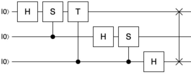
When implementing this for a number of qubits larger than three, the pattern would be the same, with each extra rotation being half of the previous one (just like $T$ is half of the rotation of $S$). We will see this later on in the Q# sample code, when implementing a four qubit QFT, where we will need half of the $T$ rotation, or, to be precise, a $\frac{\pi}{8}$ rotation.

It is worth noting that the QFT discussed in most of the subject literature, including the most popular quantum computing resource, “Quantum Computation and Quantum Information” from Nielsen and Chuang, assumes input and output to be using big endian sequencing of qubits. However, from the programmer’s perspective, little endian is usually a more natural way to reason about program’s state and therefore it is preferred in various high level quantum computing programming languages and frameworks - including Qiskit or Cirq. As a consequence, it is a common issue that when building the QFT-based quantum programs using the circuits found the quantum computing literature, one might get different result compared to when using framework-based implementations of QFT. This also explains why you may run into mirror variants of the QFT circuit in various sources.

On that front, Q# gives you an option to choose between little or big endian qubit registries on most of its operations, and indeed ships with two different built-in QFT implementations, one basing on big endian and the other on little endian registries.

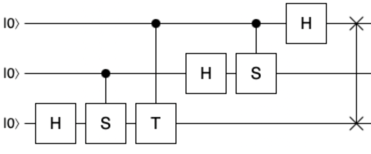
The three qubit QFT circuit relevant for little endian registry is shown below:

Q# implementation 🔗

There are two ways in which we can approach the Q# implementation for quantum Fourier transform. The manual way, by simply building the program according to the circuit we just discussed, and, if needed, scaling it appropriately to the number of involved qubits. The second approach, which is definitely the recommended and more developer-friendly technique, is to simply rely on the built-in QFT that is part of the core library of Q#. Let’s try both of these on a four qubit quantum system.

First, we will manually implement the circuit, and for that we will need to use a mixture of controlled $S$, controlled $T$ and controlled $Rz$ gates, all of which are of course part of Q#. Since we act on four qubits here, instead of the three that our circuit depicted, we have to include an additional rotation by $PI()/8.0$ radians. Additionally, moving from three to four qubits requires us to perform two, instead of only a single swap - to properly reverse the order of the qubits. The Q# code implementation is shown below.

use qubits = Qubit[4];
H(qubits[0]);
Controlled S([qubits[1]], qubits[0]);
Controlled T([qubits[2]], qubits[0]);
Controlled Rz([qubits[3]], (PI()/8.0, qubits[0]));

H(qubits[1]);
Controlled S([qubits[2]], qubits[1]);
Controlled T([qubits[3]], qubits[1]);

H(qubits[2]);
Controlled S([qubits[3]], qubits[2]);

H(qubits[3]);
SWAP(qubits[2], qubits[1]);
SWAP(qubits[3], qubits[0]);

This is everything, and it does work as expected, though we have to be aware that the implementation follows the big endian ordering here - just as it was noted when we defined the circuits. The method can be extended for more qubits using the pattern we already adopted: adding an additional halved rotations for each extra qubit, and an additional swap for every second extra qubit. At the same time, it is of course hard not to frown at such a manual approach, as it is not very maintainable, quite tedious and error prone.

The alternative is much simpler and relies on using the built in $QFT$ transformation from the core library of Q#, from the $Microsoft.Quantum.Canon$ namespace. The code is dramatically simpler and is shown below.

use qubits = Qubit[4];
let register = BigEndian(qubits);
QFT(register);

The input into to the $QFT$ operation is not a raw array of qubits, but rather a $BigEndian$ registry - similar to how it was the case in our manual implementation above. The great thing about using the built-in library functionality, is that this now scales to any number of qubits nicely, and the correctness of the implementation is guaranteed by the Q# language team.

Before we conclude for this part, we can also look at the QFT implementations that work with the little endian ordering. For the manual approach, it would mean reversing the qubits, as it was depicted on the earlier circuit diagram. The updated code is shown next.

use qubits = Qubit[4];
H(qubits[3]);
Controlled S([qubits[2]], qubits[3]);
Controlled T([qubits[1]], qubits[3]);
Controlled Rz([qubits[0]], (PI()/8.0, qubits[3]));

H(qubits[2]);
Controlled S([qubits[1]], qubits[2]);
Controlled T([qubits[0]], qubits[2]);

H(qubits[1]);
Controlled S([qubits[0]], qubits[1]);

H(qubits[0]);
SWAP(qubits[1], qubits[2]);
SWAP(qubits[0], qubits[3]);

For the library approach, we will have to call a different library function, called $QFTLE$, also from the $Microsoft.Quantum.Canon$ namespace. Naturally, in this case, the input registry must be of type $LittleEndian$.

use qubits = Qubit[4];
let register = LittleEndian(qubits);
QFTLE(register);

In each of the four cases, we can visualize the result of the transformation nicely by executing the $DumpMachine$ function from the $Microsoft.Quantum.Diagnostics$ namespace. This will only work on the simulator - after all, on real quantum hardware, we cannot inspect the state before the measurement - but it will allows us to verify that in both pairs of the implementations we are able to reach the same results.

Summary 🔗

In this post we went through the mathematical foundations for quantum Fourier transform, as well as discussed the Q# code that implemented it. The code relied both on the manual circuit execution according to the theoretical model for QFT and on the framework features provided by core Q# library. This allowed us to contrast both approach and verify that our reasoning was correct.

In the next part we will learn about some application cases of QFT.