In this post we will start exploring the topic of quantum search - the ability to locate a specific qubit state in an unsorted data set represented in a qubit register. We will look at the mathematics behind this problem, at the Q# code illustrating some basic examples and explain how the different building blocks fit together. This will help us lay ground for a more comprehensive discussion of the so-called Grover’s algorithm next time.

Background 🔗

In 1996, Indian-American computer scientist Lov Grover of Bell Labs, published a paper describing what became one of the most important algorithm in the quantum information processing theory - a search through an unsorted data set on a quantum computer. The paper, entitled A fast quantum mechanical algorithm for database search, described a hypothetical use case of searching through a phone book to find a specific phone number to find the name of a person to which this number belongs (thus, making up an unsorted set).

In a remarkable insight Grover realized, that this problem, which classically is described as having $O(N)$ complexity, can actually be solved on a quantum computer in $O(\sqrt{N})$ steps, thus achieving a quadratic speed-up.

In order to find someone’s phone number with a probability of $\frac{1}{2}$, any classical algorithm (whether deterministic or probabilistic) will need to look at a minimum of $\frac{N}{2}$ names. Quantum mechanical systems can be in a superposition of states and simultaneously examine multiple names. By properly adjusting the phases of various operations, successful computations reinforce each other while others interfere randomly. As a result, the desired phone num-
ber can be obtained in only $O(\sqrt{N})$ steps.

Grover’s algorithm made use of several innovative techniques for quantum information processing. His primary tools were the usage of phase of the amplitude to encode (“mark”) information without affecting the classical probabilities and the usage of inversion about average to convert phase differences into amplitude differences.

We will look in more detail at the precise steps of the algorithm in the next post - today let’s look at the most basic case of it, applied to an array of four numbers.

Basic theory 🔗

Imagine that we have an unsorted array of four numbers - ranging from 0 to 3, for example:

$$N = [3,0,1,2]$$

How would you find a specific number, let’s say, 2, in this array? If the collection is unsorted and unstructured in any way, using classical computing, you have to rely on a simple iterative approach - keep checking the numbers one by one and verify if it’s the one we are looking for. If we are lucky, we can find the right number on first attempt; we may also find it on second attempt. If not, then we only have 2 values left and we will surely find it on third attempt, because we will either pick the correct number, or if not then there is only other possibility and we will be certain that it contains the number we are looking for. The average amount of attempts needed before the right value is found can be expressed using probabilities in a following way:

$$1 \times \frac{1}{4} + 2 \times \frac{1}{4} + 3 \times \frac{1}{2} = 2\frac{1}{4}$$

In other words, we need on average 2.25 number checks before we find the right value in a four item array. We can also rephrase this statement into a functional problem - given a boolean verification function $f(x)$, which returns 1 (true) for a match (the selected value is indeed equal to 2) and returns 0 (false) for a miss (the selected value is not equal to 2), we need to execute the function on average 2.25 times before we can find a match.

Stated this way, the problem becomes comparable with a solution we can provide on a quantum computer and, remarkably, it can be solved there (for the aforementioned four item collection) using a single oracle function evaluation.

The four possible numbers can be binary encoded in the following way:

$$0 = 00$$

$$1 = 01$$

$$2 = 10$$

$$3 = 11$$

Since we have 4 possibilities, this also implies that in order to encode these four possibilities into a quantum computer, thanks to the superposition, we will only require two qubits, because the state space of a two qubit system is $2^2 = 4$ dimensional.

Let’s start our calculation with two qubits in the basis states $\ket{0}$.

$$
\ket{\psi_1} = \ket{0}\ket{0}
$$

Next, we will apply the $H$ transformation to each of them, or, stated differently - as we learned in the last part of this series, we apply the Walsh-Hadamard transformation $W$ to the entire system.

$$
\displaylines{\ket{\psi_2} = (H \otimes H)\ket{\psi_1} \ = \frac{1}{\sqrt{2}}(\ket{0} + \ket{1})\frac{1}{\sqrt{2}}(\ket{0} + \ket{1})}
$$

Due to linearity, we can rewrite $\ket{\psi_2}$ as:

$$
\ket{\psi_2} = \frac{1}{2}(\ket{00} + \ket{01} + \ket{10} + \ket{11})
$$

Which tells us that we have a uniform superposition of all four classical numbers $0$, $1$, $2$ and $3$ (encoded into qubits). According to the Born rule, there is now an equal 0.25 probability of receiving any one of them upon measurement. At this point we actually have all possible solutions in a superposition - and this is an important part of thinking of problem solving in quantum computing. Whatever answer our algorithm is seeking, if we have a superposition of all possible inputs into the algorithm, then the answer is already there in the quantum state space - we just need to be able to efficiently fish it out. Thankfully, as Grover found out, there are some rather clever tricks that can be used for that.

When constructing a quantum counterpart to the verification function $f(x)$, we can do it in a way that the correct result will have its phase amplified. This can be done using the controlled Z gate - $CZ$. While we covered a number of gates already in this series, we have not actually looked at $CZ$ yet, though we did discuss the single qubit $Z$ gate, and we even applied it in the quantum teleportation protocol.

To recap quickly. the $Z$ gate performs a rotation aroung the Pauli Z axis by $\pi$ radians, resulting in the so-called phase flip (sign flip) of the qubit:

$$
Z(\alpha\ket{0} + \beta\ket{1}) = \alpha\ket{0} - \beta\ket{1}
$$

Note that while the probability amplitudes in the computational basis did not get affected by the $Z$ transformation, this isn’t the case in other bases - for example in the X basis, the $Z$ gate would flip $\ket{+}$ into $\ket{-}$ state. This is actually a rather profound consequence - we can in fact reconstruct the $Z$ gate as the following:

$$
Z = HXH
$$

which can be read as - change to the X basis, flip the bit, change back away from the X basis.

The controlled $Z$ gate is the generalization of the $Z$ transformation onto a two-qubit system - as other controlled transformations, it applies the $Z$ phase flip onto the target when the control qubit is in state $\ket{1}$. As we saw above, in the single qubit case, in the computational basis, the transformation only acted on the amplitude associated with $\ket{1}$. Similarly, in the $CZ$, the only affected state is $\ket{11}$.

It is easy to notice that as it is the case with other controlled gates, $CZ$ contains the $I$ matrix in the top left corner, and the relevant target transformation matrix, $Z$ matrix in this case, in the bottom right corner.

Another interesting feature of $CZ$ is that despite the fact that it is a “controlled” gate, due to always only acting on the $\ket{11}$ state, it actually doesn’t matter which qubit is control and which one is target; the effect of the $CZ$ transformation is the same regardless.

Similarly to $Z$ gate, which can be reconstructed from a combination of $X$ and $H$, $CZ$ can be expressed as a combination of $CNOT$ and $H$:

$$
CZ = (I \otimes H)CNOT(I \otimes H)
$$

If we now use the $CZ$ gate on our state $\ket{\psi_2}$, we get the phase flip on $\ket{11}$:

$$
\displaylines{\ket{\psi_3} = CZ(\ket{\psi_2} \ = \frac{1}{2}(\ket{00} + \ket{01} + \ket{10} - \ket{11})}
$$

This means that the state $\ket{11}$ is now marked with a different phase. Even though the classical probabilities remain the same, we have a specific, unique property attached to that state now, namely its probability amplitude is negative.

This appears like something potentially useful, but not necessarily something that helps us in tackling the problem that we stated. After all, we are chasing the classical value $2$, or it’s bit representation $10$, instead of $11$ (a classical $3$). However, as we learned from part 2 of this series, we can use the $X$ gate to swap probability amplitudes in the qubit. In our case, this means applying $X$ to qubit number one:

$$
\displaylines{\ket{\psi_4} = (I \otimes X)\ket{\psi_3} \ = \frac{1}{2}(\ket{00} + \ket{01} - \ket{10} + \ket{11})}
$$

At this point in the process, we have the phase shift marking $\ket{10}$, which is actually the answer to our problem. The question is, what is the significance of that, if we still have only 0.25 probability of reading it out upon measurement? As it turns out, the remarkable trick that Grover came up with was what he called the inversion about the average (inversion about the mean). It gives us the ability to convert phase differences into magnitude (amplitude) differences. It is represented by the following sequence of operations, where $A$ denotes the entire transformation:

$$
A = (H \otimes H)(X \otimes X)CZ(X \otimes X)(H \otimes H)
$$

How does the flipping about the mean works? In our case, we have the state:

$$
\ket{\psi_4} = \frac{1}{2}(\ket{00} + \ket{01} - \ket{10} + \ket{11})
$$

That means, the four probability amplitudes are $\frac{1}{2}$, $\frac{1}{2}$, $-\frac{1}{2}$ and $\frac{1}{2}$ respectively. The sum of all amplitudes is $1$ and therefore the mean is $\frac{1}{4}$. The three amplitudes that are $\frac{1}{2}$ are currently $\frac{1}{4}$ above the mean, so in order to flip them about the mean we must change them to $\frac{1}{4}$ below the mean - so they become $0$. On the other hand the amplitude for $\ket{10}$ is actually $-\frac{1}{2}$ and thus $\frac{3}{4}$ below the mean. We need to flip it $\frac{3}{4}$ above the mean which results in $1$. The mean remains the same, the sum of all amplitudes is the same, and the relative distance to the mean is also still the same for each amplitude. However, the one amplitude we are interested in has been amplified, while the others have been reduced.

This is quite profound, because it leads it to state where we have a 100% measurement certainty of obtaining the desired state $\ket{10}$:

$$
\ket{\psi_f} = 0\ket{00} + 1\ket{01} + 0\ket{10} + 0\ket{11} = \ket{10}
$$

We can retrace this through the application of the components of the $A$ transformation we mentioned earlier.

$$
\displaylines{\ket{\psi_5} = (H \otimes H)\ket{\psi_4} \ = \frac{1}{2}(\ket{00} - \ket{01} + \ket{10} + \ket{11})}
$$

$$
\displaylines{\ket{\psi_6} = (X \otimes X)\ket{\psi_5} \ = \frac{1}{2}(\ket{00} + \ket{01} - \ket{10} + \ket{11})}
$$

$$
\displaylines{\ket{\psi_7} = CZ\ket{\psi_6} \ = \frac{1}{2}(\ket{00} + \ket{01} - \ket{10} - \ket{11})}
$$

$$
\displaylines{\ket{\psi_8} = (X \otimes X)\ket{\psi_7} \ = \frac{1}{2}(-\ket{00} - \ket{01} + \ket{10} + \ket{11})}
$$

$$
\ket{\psi_9} = (H \otimes H)\ket{\psi_8} = -\ket{10}
$$

Notice that the first two steps were really not necessary in this simple case - because $\ket{\psi_4}$ is equal to $\ket{\psi_6}$, but as we will see in the next post, they will be needed for more complex cases. At the end we are left with 100% probability of reading out a state $\ket{10}$ in a single measurement - which is our classical number $2$ that we needed to find.

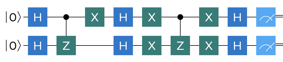
This a terrific example of a quantum comptutational speed up - we went from an average of 2.25 classical evaluation steps to a single quantum measurement step. The overall circuit depicting our theoretical model is shown below:

Q# implementation 🔗

Let us now shift our attention towards the demonstration of this simple quantum search program in Q#. This should not be too difficult, given that we already have a reference circuit.

We will call our Q# operation $TwoQubitFixedSearch$, and in it we will allocate two qubits. Then we simply follow the sequence of gates defined in the circuit. While this is not always the case in quantum frameworks, there actually is a built-in two qubit $CZ$ gate in Q#, which we can take advantage of.

operation TwoQubitFixedSearch() : Int {
    use (q1, q2) = (Qubit(), Qubit());

    // superposition
    H(q1);
    H(q2);

    // CPHASE or CR(π), only flips the phase of |11>
    CZ(q1, q2);
    DumpMachine();

    // swap phase change to state -|10>
    X(q1);

    // invert about the mean
    H(q1);
    H(q2);
    X(q1);
    X(q2);
    CZ(q1, q2);
    X(q1);
    X(q2);
    H(q1);
    H(q2);

    // measure as integer
    let register = LittleEndian([q1, q2]);
    let number = MeasureInteger(register);
    return number;
}   

Since we explicitly want to mark the state $\ket{10}$, we perform the extra $X$ transformation on qubit one after the $CZ$ phase change. One extra feature we take advantage of here, is the ability to create a so called QPU register, a $LittleEndian$ reigster and measure it directly into an integer using $MeasureInteger$ operation from the $Microsoft.Quantum.Arithmetic$ namespace. This convenience feature of Q# simplifies the process of performing arithmetic calculations on the quantum processing unit. It also takes care of resetting qubits, which no longer needs to be done manually in this case.

The remaining step is to add the code that will act as the program’s entry point and that will invoke our simple search algorithm.

@EntryPoint()
operation Main() : Unit {
    let result = TwoQubitFixedSearch();
    Message($"Expected to find a fixed: 2, found: {result}");
}

Since the program is hardcoded to mark the state $2$ as the one to find, not surprisingly, it also finds $2$. This will be demonstrated by the output:

Expected to find a fixed: 2, found: 2

Before we close this off, we can still create a slightly more generic variant of the code, that will allow us to test search for all four possible values from $0$ to $3$ - in order to verify that we didn’t make a mistake in our theoretical work. This generalized variant for the two qubit, four value set is shown below as a $TwoQubitGenericSearch$ operation.

operation TwoQubitGenericSearch(numberToFind : Int) : Int {
    use qubits = Qubit[2];

    // superposition
    ApplyToEachA(H, qubits);

    // CPHASE or CR(π), only flips the phase of |11>
    CZ(qubits[0], qubits[1]);

    // swap phase change to desired state
    if (numberToFind == 1 or numberToFind == 0) {
        X(qubits[1]);
    }
    if (numberToFind == 2 or numberToFind == 0) {
        X(qubits[0]);
    }

    // invert about the mean
    ApplyToEachA(H, qubits);
    ApplyToEachA(X, qubits);
    CZ(qubits[0], qubits[1]);
    ApplyToEachA(X, qubits);
    ApplyToEachA(H, qubits);

    let register = LittleEndian(qubits);
    let number = MeasureInteger(register);
    return number;
}

This operation takes in an integer as input, which allows us to pass in different marker values. In order to improve the readability of the code, we now no longer invoke each gate individually on each qubit, but use the $ApplyToEachA$ helper operation wherever possible. To make this possible, instead of allocating the qubits individually, they are now allocated into a single array.

Depending on the number needed to be marked, no $X$ gates are invoked ($3 = \ket{11}$), $X$ is invoked on qubit one like in the previous example ($2 = \ket{10}$), $X$ is invoked on qubit two ($1 = \ket{01}$) or it is invoked on both qubits ($0 = \ket{00}$). The rest of the algorithm is the same as it was before.

We can now invoke this code covering all four cases:

@EntryPoint()
operation Main() : Unit {
    for i in 0..3 {
        let found = TwoQubitGenericSearch(i);
        Message($"Expected to find: {i}, found: {found}");
    }
}

When executed, the program should produce the following output:

Expected to find: 0, found: 0
Expected to find: 1, found: 1
Expected to find: 2, found: 2
Expected to find: 3, found: 3

Summary 🔗

In this post we looked at the simplest possible variant of quantum search protocol based on Grover’s algorithm. We discovered that it can solve, in a single shot, a problem that takes on average 2.25 iterations on a classical computer. At the same time, in order to ease ourselves into the theory, we purposely didn’t wander beyond two qubits / four values case - however, there is no need to worry; this is something we will do in the next part of this series.