Some years (wow, time flies!) ago I wrote a quantum computing book titled “Introduction to Quantum Computing with Q# and QDK” (I guess it’s difficult to miss too, since its cover still sits in the sidebar of this blog…). Even though a ton of things have changed in QDK since than, I have been maintaining the source code throughout the years - most importantly, porting everything to QDK 1.0.

Today I would like to share yet another update: the samples are now also available as Jupyter notebooks.

Notebooks alongside standalone Q# files 🔗

Each sample in the repository now ships with a companion demo.ipynb notebook, sitting next to the original Program.qs file. The two files are deliberately kept separate, and that separation is in fact the central design decision behind this update.

The Program.qs file contains pure Q# code. It is written as a self-contained quantum program - one that can be opened, inspected, have its circuit generated and executed entirely on its own within VS Code using the QDK extension. The Q# operations directly model the quantum mechanics discussed in the book: entanglement, interference, measurement, and the various quantum algorithms across the chapters. There is no Python, no orchestration logic, no classical bookkeeping embedded in there.

The notebook then acts as a classical driver for those same quantum operations. Using the qsharp Python package, it loads the .qs file at runtime, makes all of its operations available as regular Python callables through the qsharp.code namespace, and from that point handles everything classical: running multiple shots, collecting statistics, computing derived quantities, and producing visualisations. This includes shot orchestration: the Q# operations are single-shot by design, and the notebook decides how many times to invoke each one and how to aggregate the results. For example, in the Bell inequality sample, the Python layer is responsible for estimating correlators across thousands of measurement runs and computing the CHSH value - while the actual quantum circuit preparation and measurement is entirely defined in Q#.

Why this separation matters 🔗

The key motivation here is pedagogical. The book has always tried to present quantum computing from two complementary angles simultaneously - the mathematical and the programmatic. While it is possible to do everything in Q# (like the original samples did), the notebook may be preferred to some, as it creates a clear quantum-classical boundry. A reader can study the Q# file to understand the quantum mechanics of a given protocol in isolation, without any classical noise around it. They can then open the notebook to see how the same operations are used as building blocks within a richer classical context, and observe the statistical outcomes that emerge from repeated quantum sampling.

The Q# programs are not entangled with the notebook runtime - they can just as easily be submitted to Azure Quantum or run from a plain Python script. The notebook is just one possible classical host, and treating it as such keeps the responsibilities cleanly separated.

There is one more practical benefit worth mentioning. Each Q# file remains a runnable program in its own right - the presence of a Main operation means you can always execute it directly from the command line or the VS Code integrated runner, without ever touching the notebook. This makes the samples useful across different preferences and workflows.

Example 🔗

Below is the practical example, using quantum teleportation.

The original code (ported to QDK 1.x already) used 4096 shots inline in Q#, and simply printed the message about the resulting success rate:

import Std.Convert.*;
import Std.Math.*;

operation Main() : Unit {
    let runs = 4096;
    mutable successCount = 0;

    for i in 1..runs {
        use (message, resource, target) = (Qubit(), Qubit(), Qubit());

        PrepareState(message);

        Teleport(message, resource, target);
        Adjoint PrepareState(target);
        set successCount += M(target) == Zero ? 1 | 0;
        ResetAll([message, resource, target]);
    }

    Message($"Success rate: {100. * IntAsDouble(successCount) / IntAsDouble(runs)}");
}

operation Teleport(message : Qubit, resource : Qubit, target : Qubit) : Unit {
    // create entanglement between resource and target
    H(resource);
    CNOT(resource, target);

    // reverse Bell circuit on message and resource
    CNOT(message, resource);
    H(message);

    // measure message and resource
    let messageResult = M(message) == One;
    let resourceResult = M(resource) == One;

    // and decode state
    DecodeTeleportedState(messageResult, resourceResult, target);
}

operation PrepareState(q : Qubit) : Unit is Adj + Ctl {
    Rx(1. * PI() / 2., q);
    Ry(2. * PI() / 3., q);
    Rz(3. * PI() / 4., q);
}

operation DecodeTeleportedState(messageResult : Bool, resourceResult : Bool, target : Qubit) : Unit {
    if not messageResult and not resourceResult {
        I(target);
    }
    if not messageResult and resourceResult {
        X(target);
    }
    if messageResult and not resourceResult {
        Z(target);
    }
    if messageResult and resourceResult {
        Z(target);
        X(target);
    }
}

The notebook variant relies on the following (very similar) Q# code, but without any orchestration:

import Std.Math.*;

operation Main() : Unit {
    let result = RunTeleportation();
}

// Returns Zero if teleportation succeeded
operation RunTeleportation() : Result {
    use (message, resource, target) = (Qubit(), Qubit(), Qubit());
    PrepareState(message);
    Teleport(message, resource, target);
    Adjoint PrepareState(target);
    let result = M(target);
    ResetAll([message, resource, target]);
    return result;
}

operation Teleport(message : Qubit, resource : Qubit, target : Qubit) : Unit {
    H(resource);
    CNOT(resource, target);

    CNOT(message, resource);
    H(message);

    let messageResult = M(message) == One;
    let resourceResult = M(resource) == One;

    DecodeTeleportedState(messageResult, resourceResult, target);
}

operation PrepareState(q : Qubit) : Unit is Adj + Ctl {
    Rx(1. * PI() / 2., q);
    Ry(2. * PI() / 3., q);
    Rz(3. * PI() / 4., q);
}

operation DecodeTeleportedState(messageResult : Bool, resourceResult : Bool, target : Qubit) : Unit {
    if not messageResult and not resourceResult {
        I(target);
    }
    if not messageResult and resourceResult {
        X(target);
    }
    if messageResult and not resourceResult {
        Z(target);
    }
    if messageResult and resourceResult {
        Z(target);
        X(target);
    }
}

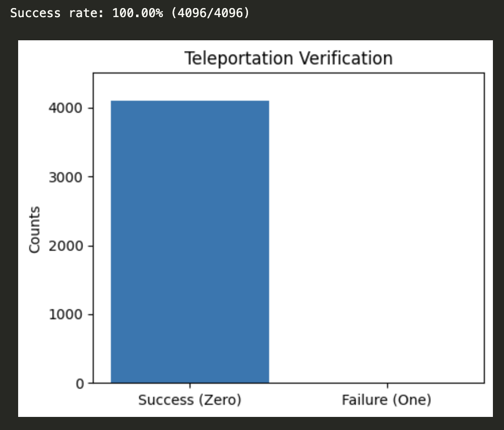
Shot orchestration is now done from Python:

shots = 4096
results = [str(RunTeleportation()) for _ in range(shots)]
successes = results.count("Zero")

print(f"Success rate: {successes * 100 / shots:.2f}% ({successes}/{shots})")

fig, ax = plt.subplots(figsize=(5, 4))
ax.bar(["Success (Zero)", "Failure (One)"], [successes, shots - successes])
ax.set_ylabel("Counts")
ax.set_ylim(0, shots * 1.1)
plt.title("Teleportation Verification")
plt.show()

This of course allows creating a visualization too:

Getting the samples 🔗

The notebooks can be found in the book source code repository, on the notebook-orchestration branch. The Python dependencies required to run them are listed in requirements.txt at the root of the repository. I hope you find them useful - and as always, happy Q#-ing!